Marc Kassis, Robert Kibrick, Connie Rockosi, Gregory D. Wirth
Revised January, 2011
Contents
- Background
- Red Dewar Characteristics
- Performance
- Detector Operation
- Dealing With Images
- Observing Strategies
- Additional Notes
Background
In December 2010, WMKO and UCO/Lick installed and commissioned LRIS Red III (Mark II Upgrade) with a new detector mosaic. This mosaic was fast tracked to the telescope to replace the failing mosaic (see the news pages for details on the charge transfer efficiency problems). The upgrade addresses the detector problems that have impacted observers since Oct 2009.- The following attributes remain the same
when comparing the original detector to that of LRIS Red III.
- high quantum efficiency in the red, extending coverage into the I band;
- elimination of interference fringes and the associated problems with flat-fielding resulting from image motion due to instrumental flexure;
- larger detector area for greater spectral range;
- smaller pixel size;
- flat focal plane for more uniform focus across the red field of view.
Red Dewar Characteristics
Physical Description
The new LRIS-R mosaic (LRIS Red III) consists of two 2k×4k LBNL high-resistivity CCDs. The two devices installed are identified as 19-2 and 19-3. CCD 19-3 is sensitive to temperature, and as a result, both CCDs are operated at -99 �C (relative to -140 �C for the original upgrade). The warmer operating temperature thus increases the overall noise of the system, but does improve the QE relative to the existing mosaic.These devices still offer significantly higher quantum efficiency (QE) in the red over the original detector,extending the usable wavelength range of the red side of LRIS into the I band. Plots of the QE curves for each device in the mosaic are attached later in this document. In addition, images taken with these CCDs do not suffer from interference fringes, thus reducing the impact of instrumental flexure on flat field corrections.
In this document, we use the following nomenclature to differentiate between the past and current systems.
- LRIS Red I: original 1994 dewar with Tektronix/SITE 2k×2k CCD
- LRIS Red II: 2009 2x(2kx4k) LBNL mosaic and dewar
- LRIS Red III: 2010 2x(2kx4k) LBNL mosaic and dewar
In comparison to LRIS Red I, these CCDs provide a larger detector area, smaller pixels (15 μm versus 24 μm in the Tektronix/SITE 2k×2k CCD), and a flatter focal plane. Because the area per pixel is now 40% of what it used to be, observers are encouraged to bin pixels during CCD readout, and both row and column binning are supported.
These CCDs have some traps, cosmetic defects, and other anomalies. These foibles are described in the accompanying section on cosmetics.
Detector Characteristics
Quantum Efficiency
The quantum efficiency curves as measured in the lab at Lick are presented below. As a result of operating the CCDs at a warmer temperature than LRIS Red II (-100 vs -140 C), the QE is slightly better in the far red. The QE curves below are taken from the "LRIS-R Test Report:LBNL High Resistivity CCDs 19-2 and 19-3" supplied to Keck on 17 Aug 2010. The QE for 19-2 was not measured at the current operating temperature, and there is a slight improvement in the QE at the longest wavelengths for an operating temperature of -100C. The QE for 19-3 was measured at the operating temperature.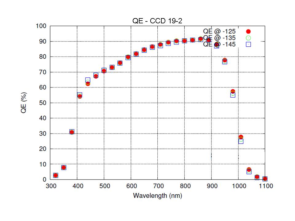
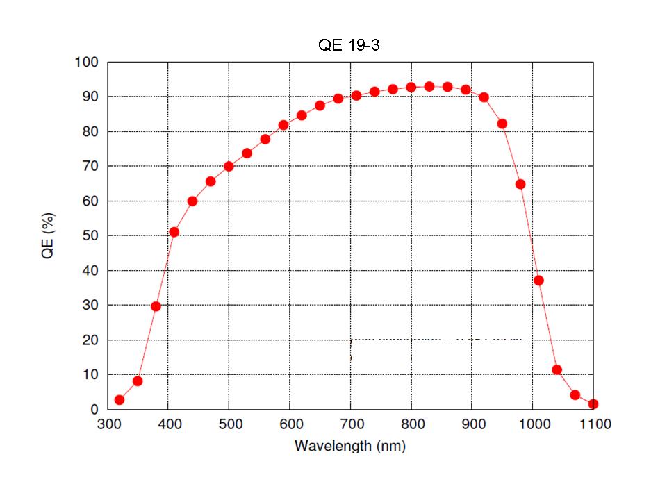
QE for CCDs 19-2 (left) and 19-3 (right).Gain & Readnoise
Under normal operations, observers will use "normal" CCD speed with the gain set to "high" while binning 1x1, 1x2, 2x1, or 2x2. For graphs and files providing latest gain and readnoise measurements see the gain and readnoise documentation.Readout Times
The new red mosaic offers three readout speeds but only one is used for observing.- Normal. The default observing mode, it provides a compromise between speed and readout noise. At "normal" readout speed, the new mosaic takes longer to read out than LRIS Red I and II.
- Fast. Uncharacterized. But it does work and is available for use.
- Slow. Uncharacterized.
*Elapsed time for 0 sec exposure, including erase, expose, and readout phases.LRIS-R Mosaic Readout Times CCDSPEED Binning Readout Time (s)* Normal 1x1 127 Normal 1x2 (spectral) 78 Normal 2x1 (spatial) 83 Normal 2x2 58 Linearity
In contrast to LRIS Red I, the onset of non-linearity occurs before the saturation of the ADC. Observers should strive to keep the peak signal level below 38,000 DN to ensure that they are operating in the linear regime. Below is a plot that shows the linearity of the four amplifiers.
Linearity fo rthe four readout regions.The image below shows the layout of the four LRIS Red III video amplifiers as the image is displayed in DS9 when observing. The observational setup for DS9 rotates the images by 270 degrees to place the bluest wavelengths on the left of the image and the reddest on the right. The location of the longslit spectrum (yellow line) lands on vid 4 when the object is placed at the standard "slitb" pointing origin.
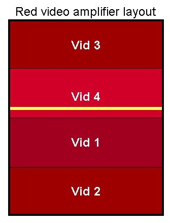
LRIS Red III amplifier layoutCosmetics
The number of cosmetic defects on CCDs 19-2 and 19-3 are comparable to the to those of the previous detector. Instead of the "tape effect" and low level traps, the new CCDs have hot defects, traps, and glue voids to contend with. Below is an image of a flat with overlays of the cosmetic defects. The image is color coded:- yellow lines - traps and hot pixels with tails
- red lines - column channel stop failures
- green plus - Clusters of hot pixels or traps
- Shaded green - Glue voids
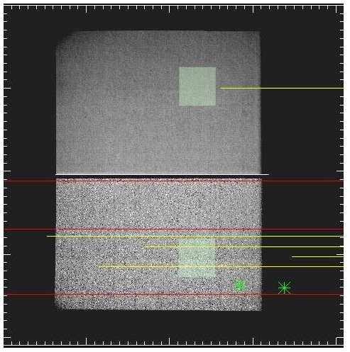
Map of Cosmetic DefectsHot Pixels and Traps
Below is a table that describes the locations of hot pixels and traps. In some cases, the hot pixels and traps have a long tail associated with it.
Location hot pixels and traps.CCD DS9 Pane Coordinates Notes X pix Y pix 19-2 3906 3627 Hot pixel 19-2 3406 2878 Trap cluster 19-2 3375 2850 Trap 19-2 3796 3545 Trap with tail 19-3 1314 526 Hot pixel with tail 19-3 1188 1706 Hot pixel with tail 19-3 1065 3471 Hot pixel with tail
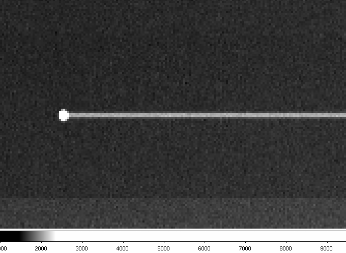
Magnified view of a hot pixel with a tail.Column channel stop failures
Columns in the CCD are defined by potential barriers that keep charge in one column from combining with neighbors, and the barriers are usually referred to as column stops. On CCD 19-3, there are three places where the column stops have appeared to break down, and charge has spilled into the neighboring columns. Below is a table which lists where the channel stop failures are located. These channel stops are mapped on the above image in red. Below the table, a figure shows the average row plots for the channel stop failure columns.
Location of failed channel stops.CCD DS9 Pane Coordinates X pix Y pix 19-3 1979-1980 0-4096 19-3 1395-1396 0-4096 19-3 613-615 0-4096
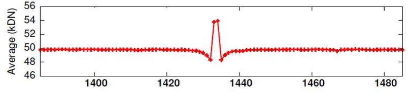
An example average row plot for a failed channel stop.Glue Voids
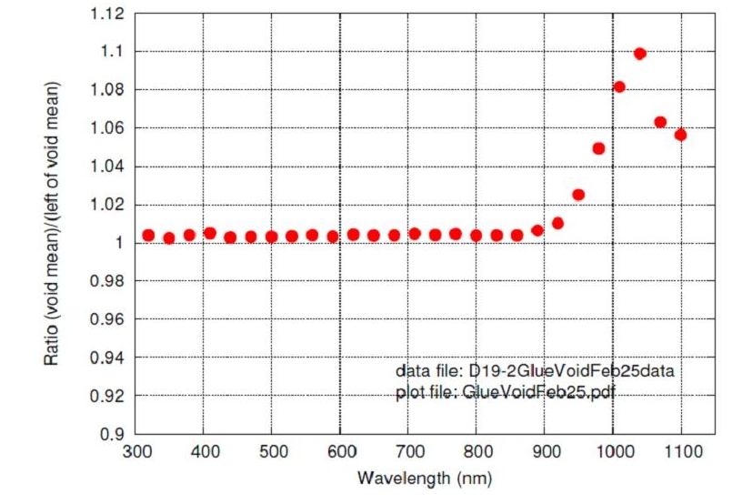
The figures below show the magnified views of the "glue voids" that are present on both halves of the mosaic. At most wavelengths, observers will only detect the edges of the glue void which manifest themselves as a dark interior band a pixel or two wide and a lighter band exterior to the dark band. We suspect that the banding arises from a redistribution of charge, with some of the charge moving from the dark pixels into the lighter pixels.So far, flat-fielding appears to correct for the glue voids at all wavelengths. However, because the edge of the void redistributes charge, objects or spectral features spanning the edge may be distorted. special care should be taken when measuring position or extracting spectra at the edges of the glue void.
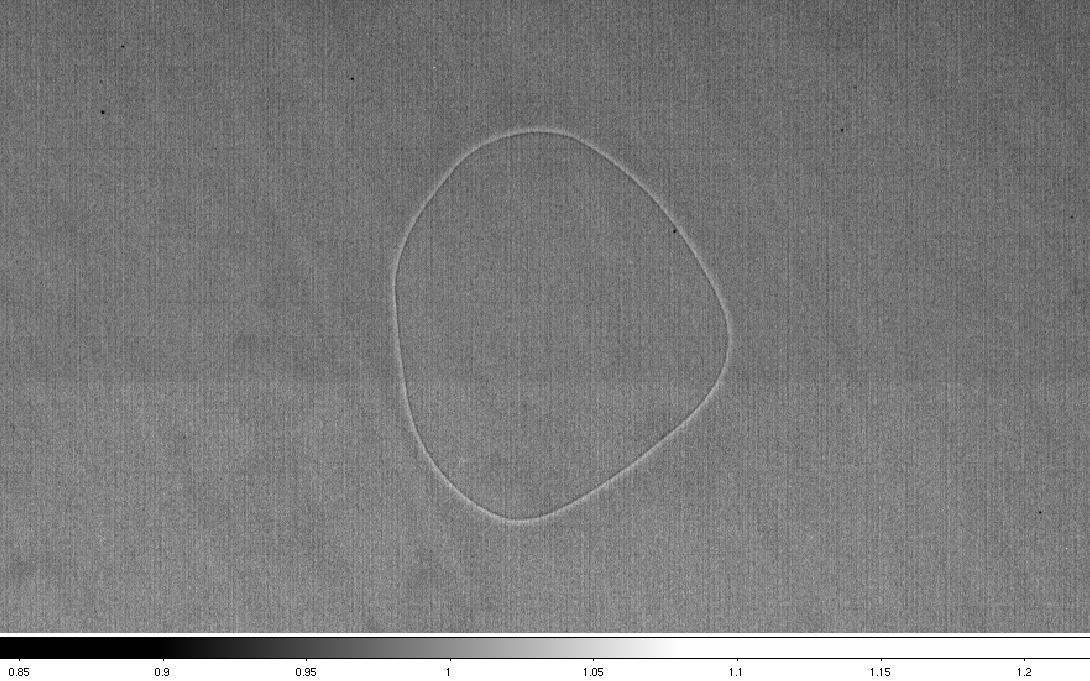
Glue void for 19-2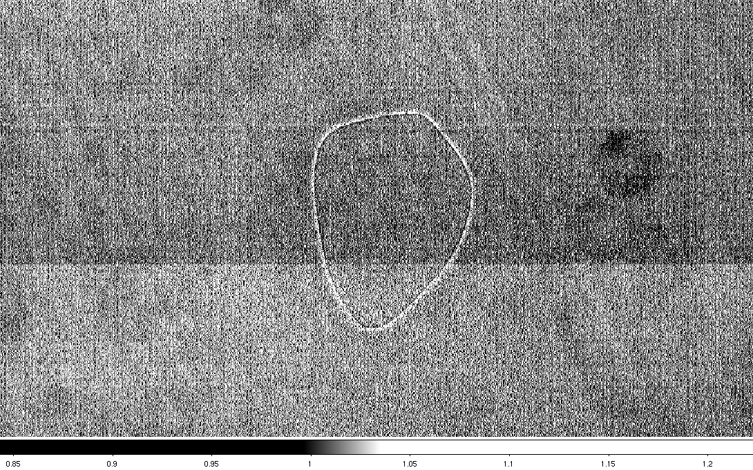
Glue void for 19-3At wavelengths longer than 900nm the CCD is becoming optically thin so that some light passes through the detector. Because the void is an air pocket, the response relative to the rest of the CCD is diminished. Below is a plot that characterizes the response relative to the rest of the CCD.
Relative response of the glue void relative to the rest of the detector.Radiation events
The new CCDs are good cosmic ray event detectors, which is a nice way of saying that observers can expect to see the same rate of cosmic ray events in their images compared to LRIS Red II (higher than the detection rate for LRIS Red I). The rate of cosmic ray and other radiation events is such that in a 1200 second dark exposure, between 0.7% and 1% of the pixels are contaminated at a level more than 5σ above the background bias. The expected muon rate, taken from work done by the LBL group, Stover and others (e.g., Smith et al. 2002, Proc. SPIE, 4669, 172) in the process of characterizing these fully-depleted, thick CCDs, is about 390 events per quadrant of the mosaic. That suggests an average size for the trails of 100 pixels. The actual distribution of event sizes in pixels is extremely broad, but 100 is reasonably close to the mean. The majority of the tracks are straight, indicating that the shielding is doing its job of keeping out local low-energy electrons. An example of part of a frame is seen below.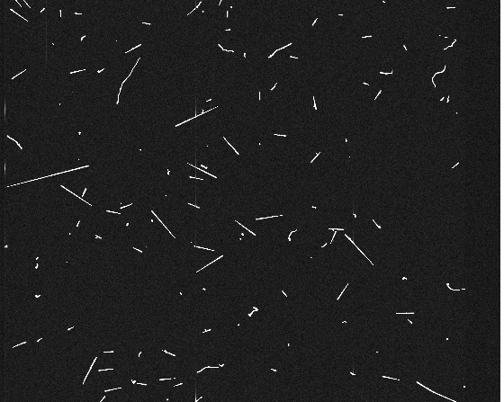
Cosmic Rays in an LRIS-R Dark Image for LRIS Red IIImage Quality
The minimum FWHM at best focus for imaging and longslit mode is comparable to that seen on the blue side. The 100 µm gradient seen in the focus in the spatial direction in the LRIS Red I is considerably less steep. A direct comparison will require more work to distinguish changes to the focus software from changes to the data. We will also analyze longslit focus data to check the image quality in the new detector real estate. The bottom line from the analysis so far is that image quality is, at worst, unchanged.Geometry
Comparison to LRIS Red I
Steve Allen of UCO/Lick has kindly produced the following diagram comparing the area of the new mosaic (shaded region) to the previous red-side CCD (white outline). This is unchanged for both upgrades.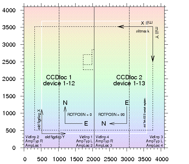
LRIS-R Science Mosaic GeometryAstrometry
Gap
The open cluster m67 was observed, and we measured the astrometry on the two sides of the mosaic. CCD 19-3 is slightly tilted relative to 19-2. The gap, specifically the distance between the first column of the two red CCDs, is at pixel Y=0 is 27.30 arcsec and at Y=4096 is 30.25 arcsec.Performance
On 16 Dec 2010, observations were acquired with LRIS Red III during engineering time. These observations included imaging with the V & I filters and slitless spectroscopy of spectroscopic standard stars. In the two sections below, we describe the reduction and measured performance in both imaging and spectroscopic modes.Zero Points
The photometric standards in m67 (Yadav, et al. 2008, A&A, 484, 609) were used to measure the zero points for the V and I filters. The cluster was observed at the LRIS pointing origin with central coordinates of 08:51:24.0 +11:48:28.0 J2000 with a PA of 90 degrees. 20s exposures were acquired, and images were divided by a flat field. Standard IRAF routines were used to identify stars, measure the flux from the source, and subtract a background. In the table below, the number of stars identified and used to calculate the average zero point is presented in the first column, followed by the mean, median, and 1 sigma uncertainty. Observations were obtained at an airmass of 1.1. At V and I bands, the measured zero points are ~0.4 magnitudes fainter than those measures with the LRIS Red I.
Measured Zero PointsFilter N-stars ZP-mean ZP-median 1 sigma I 16 27.80 27.81 0.09 V 40 27.86 27.86 0.02 Detector Operation
Windowing
Unlike the blue CCD mosaic, the red CCD mosaic may be set to read out any desired rectangular region. Windowing is now accomplished using the PANE keyword. Observers can modify the PANE keyword directly either by updating the keyword via the command line or using the window selection on the Xpose GUI. Windowing the CCD in the spatial direction will not save readout time. Windowing the CCD in the spectral direction will save time, but will reduce wavelength coverage and thus is not typically something the observer wants to do.On the CMD... menu available on the red Xpose GUI, there are options for windowing the CCD:
- Window full frame is used to readout the entire detector.
- Window longslit is used to read out only the long slit region. As noted above, this is not any faster than fullframe readouts but will save disk space.
Binning
Observers should bin the detector in the spatial and/or spectral direction for two reasons:- First, to be sky noise dominated in the same amount of time at 7000 Å as the LRIS Red I, it is necessary to bin by two in either axis.
- Second, binning decreases the readout time (see readout times).
If binning is not set to one of these standard modes, then the amplifier offsets and pixel delay clock will need to be re-tuned to minimize pattern noise for the desired configuration. This is a time consuming process and should be avoided until we have an opportunity to calibrate additional readout modes.
Observers should never modify binning using the WIN... option on the Xpose GUI, because doing so will not adjust the pixel delay clock and hence pattern noise will occur in the images. Instead, binning should only be changed using the options available on the CMD... menu.
Dealing With Images
Old vs. New Format
With LRIS Red I, the FITS files written for both the red and blue sides were written as simple FITS format with all data assembled into a single 2-D array. To comply with accepted standards for storage of CCD mosaic image data, LRIS red and blue images are now storage as multi-HDU (header data unit) FITS files. As with HIRES and DEIMOS, data from each CCD amplifier are stored in a separate image extension. Each extension includes both data and a header describing the content of that extension. Furthermore, a primary HDU contains information common to all extensions (e.g., LRIS mechanism keywords).Displaying images
The simplest way to display LRIS multi-HDU images is to read them into a FITS viewer which understands how to assemble mosaic data into an image. The ds9 image display tool is one such program. To view an LRIS image in ds9, simply open the image using the File > Open Other > Open Mosaic IRAF.. function. Note that you must set the ds9 flip and rotation parameters as follows in order to achieve the customary view which puts the spectral direction increasing to the right: [TBD] [TBD: note old vd. new ds9 difference]IRAF users may use the lrisdisplay task in the keck.lris to view images on the IRAF display tool.
IDL users can use the readmhdufits routine to read the image into a 2-D array, then display it using the atv image display tool.
Reading images (IRAF/IDL)
WMKO has made available two software tools which will generate a monolithic single-HDU image (i.e., one that combines the pixels from all amplifier regions into a single-HDU FITS file) from a multi-HDU LRIS mosaic image:- readmhdufits is an IDL routine which reads in the multi-HDU LRIS images and assembles them into a single 2-D array, with optional bias subtraction based on the overscan region.
- multi2simple is a task distributed as part of the keck.lris package to read in multi=HDU images and output a simple FITS image.
- splitmos is a utility that will convert a multi-HDU FITS file into a set of a single-HDU format files, with one file per readout amplifier region. This program is installed on the LRIS host computer.
Observing Strategies
- afternoon calibrations
- science acquisition
Send questions or comments to:LRIS Support