Contents
-
Comparison to other Keck instruments
-
Detector
-
Imaging
-
Spectroscopy
-
Guiding, Chopping, and Seeing
-
Software and User Interface
-
Data and Analysis
Comparison to other Keck instruments
Although the full answer depends on your specific needs, in general LWS
is quite competitive with OSCIR and MIRLIN. The relative capabilities of
the three instruments are shown in
this table.
For most objects you will find NIRC to be more efficient, mostly because
the InSb detector used by NIRC has much greater quantum efficiency at 3-5
µm than does the Si:As array used in LWS. However, there remain two
situations where LWS would be preferable:
-
Bright source. If the source has extremely high flux it may saturate
NIRC, yet be on scale with LWS due to the low LWS QE.
-
Extended source. With NIRC, one must read out a subarray in order
to prevent saturating the detector in the mid-IR; depending on the filter,
you may be limited to reading out a small image section with very little
resultant sky coverage. Under these circumstances, LWS may allow you to
obtain wider field-of-view than NIRC.
Detector
No. The original LWS lacked a thermal control system, thus allowing the
detector temperature to fluctuate by up to 3°K depending on the dewar
attitude (elevation). Because the quantum efficiency and gain (
etaG)
of BIB detectors is strongly temperature dependent, the response of the
original LWS thus varied with elevation. The new LWS detector no longer
has an attitude (elevation) dependence due to a precision closed-loop thermal
control system which maintains the detector at its optimum operating temperature
of 8.50±0.02 K.
Imaging
There are 4 filters currently installed in LWS for use in the 20 µm
wavelength regime. The broadband 17.9 µm ( 2.0 µm wide) filter
is recommended for imaging in the 20 µm region. This filter has good
transmission properties and is the most sensitive in this region. Another
choice is the narrow 18.7 µm ( 0.4 µm wide) filter. The
18.7 has poor transmission and is not very sensitive, however, it provides
an alternate choice during marginal weather conditions. There
are two other filters that do not have the proper diameter for use in LWS,
the 20 and 22 µm ( 2.0 µm wide) . These filters
are undersized and only transmit about 50% of the LWS beam, which effects
the sensitivity and point spread function (PSF). They have been temporarily
installed for testing and help extend the wavelength coverage for users
that need measurements in this region. The 20 and 22 µm filters are
NOT recommended for typical LWS programs.
Spectroscopy
A flux of 150 mJy in LRES (R=100) mode, or 500-1000 mJy in HRES (R=1200)
mode, yields S/N=1 per spectroscopic resolution element in 1 second
on
source. The LRES estimate assumes you are using:
-
the small (3 pixel = 0.25 arcsec) slit;
-
the low-resolution grating;
-
the broadband "N" (8-13 µm) filter;
-
central wavelength of 10 µm;
-
chop-nod observing mode.
Quoted flux is light incident on telescope. Also see the next item...
About 25%. A peculiar software feature requires us to wait an integral
number of frames for the chop motion to settle. Thus, if your frame time
is 0.5 s you must wait 0.5 s after the chop, (tossing this frame) then
take a single 0.5 s frame, cutting effficiency. The alternate which may
be acceptable sometimes is to wait zero frames after the chop and take
the hit in the psf in return for higher efficiency.
Because LWS does not have a slit-viewing guider, LWS must be placed into
imaging mode in order to position the target on the slit. In a nutshell,
the procedure is:
-
Reconfigure LWS for imaging (mirror in, imaging filter in, slit out)
-
Image the target and measure centroid
-
Insert the desired longslit
-
Image the slit and measure centroid
-
Move the target to the location of the slit center
-
Image the target in the slit and manually tweak centering using handpaddle
-
Reconfigure LWS for spectroscopy (grating in, blocking filter in)
More detailed instructions are available on the
Target
Acquisition: Spectroscopy Mode checklist.
Guiding, Chopping, and Seeing
In the near-IR (3-5 µm) LWS and NIRC will give roughly the same image
quality, typically 0.3-0.5 arcsec FWHM. In the mid-IR (10-20 µm)
LWS generally provides diffraction-limited images at FWHM=0.28 arcsec.
Seeing can degrade a little when guiding/tracking isn't so good, but is
usually 0.3 arcsec FWHM or so.
Thus far in the commissioning of LWS spectroscopy modes, keeping an object
in the 0.25 arcsec (~3 pixels) slit has not been a problem. In other words,
over periods of ~30 min the guide performance has met the requirements
for spectroscopy. Another test, designed to look for rotation-dependent
flexure, showed the long-term guide performance to be better than 0.3 arcsec.
The test duration was 3 hours while crossing the meridian within 5°
of zenith. Since this is such a critical parameter, more tests will be
performed to measure differential flexure with different gravity vectors
acting on the instrument and guider (
i.e., lower elevation). Reasons
for improvement from the old system is attributable to the LWS mounting
hardware being redesigned to make the instrument more rigid in the Forward
Cassegrain Module (FCM). Also, there is a new guide algorithm in use at
Keck that may be less sensitive to chopping effects on the guide star PSF.
At Keck, "chop-nod" mode is defined as using a secondary chop throw and
telescope nod throw of equal amplitudes but of opposite directions, 180°
apart. The result is that for each nod position one of the other chop beams
is in the same xy location (within the accuracy of the telescope guiding/tracking
system, typically 0.06" radial RMS) on the detector. For LWS, if the chop-nod
throw amplitude is greater that 5.2" then the opposite chop beam will be
off the detector (assuming your chop direction is aligned with detector
rows; if you chop at a 45° angle relative to the detector "up" direction,
you can stretch this to about 7 arcsec).
It might seem that nodding 90° from the chop and keeping all four
beams on the detector (defined as "quad-chopping") would increase the signal-to-noise
ratio (S/N). However, analysis shows that there is no gain in S/N (for
the same elapsed time) from using "quad-chopping" versus using "chop-nod".
See proof. This is counter-intuitive
since quad-chopping increases the exposure of the object on the detector
by factor 2 for an equivalent amount of time. However, quad-chopped data
requires 4 additional shift and add steps in the image processing. This
increases the background noise by sqrt(4) resulting in the same signal
to noise ratio as equivalent chop-nod data.
The guide camera and LWS are fixed in different locations of the forward
Cassegrain module, FCM. The rotation of the FCM causes circular motion
of the guide camera relative to LWS. The center of the guide camera is
432 arcsec from the center of the LWS field of view. The guide camera is
about 60 arcsec wide in this dimension so that is the width of the annulus
for available guide stars. The sky position angle between the science object
and the guide star is the angle the telescope control software uses as
an input for rotation ( note: this is different from the resulting PA for
LWS images, in other words, this is the angle you tell the OA. The limiting
magnitude, based on almost any DSS object being suitable, is about 18v
under typical seeing conditions. A tool called sky is available for making
guide star selections relatively easy and can be used during the afternoon
preparations or the OA can use it in real time without much of an overhead
penalty.
Chop-nod is the standard mode of data acquisition for LWS. Chopping
is performed to cancel out sky radiation and nodding of the telescope is
performed to help cancel out the radiation contribution from the telescope.
The LWS chop-nod style uses a nod throw equivalent to the chop throw but
in opposite directions.
See figure. The resulting
image, after double difference process, requires no further shift and add
processing. The chop-nod technique is very effective at canceling out background
radiation.
In imaging mode the efficiency can approach 50%; in spectroscopy mode it
is closer to 25%. The reason for this is that the data acquisition system
forces us to discard at least one frame during each chopper transition.
For imaging, the frame times are short (10 millisec or more) and the losses
are small. For spectroscopy, frame times must be increased in order to
reach the background-noise-limited regime (100-400 millisec) and hence
the losses are much more significant. We are working on a fix, but it involves
very low-level reprogramming of the electronics and will take some time
to complete.
Software and User Interface
Yes, the problems previously suffered by the LWS software during its first
use in 1996 have been corrected. Of course, no software is perfect and
although the LWS software still has some "features" that need improvement,
its reliability has improved vastly from earlier versions. Software crashes
have not been a significant problem during the commissioning of the new
LWS. The few crashes we have observed occurred when LWS was operating in
a "free running" video mode, as opposed to the data-saving mode employed
during observing. After several hours in this video mode the acquisition
software has a tendency to crash, but the recovery time is typically less
than 2 min.
It should be noted that the old LWS system also had a hardware problem
which caused spontaneous rebooting, a factor that helped lead to its de-commissioning.
This problem is now corrected and not one occurrence of the "spontaneous
reboot" has occurred during the LWS re-commissioning.
Data and Analysis
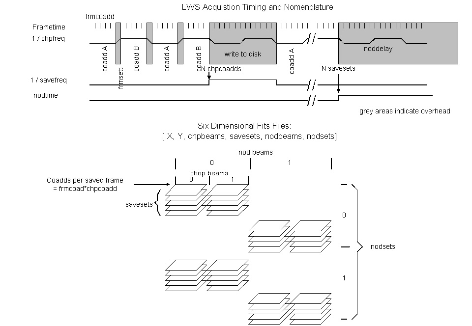
The LWS data acquisition system allows the user a choice in setting up
the various parameters that determine the FITS file dimensions. In particular
the user can select a save-to-disk frequency (maximum
5 Hz)
. The save frequency and the total integration time determine the chop
sets (sometimes referred to as savesets) and nod sets (see below). A higher
save frequency may allow the user to apply "shift and add" or other techniques
in order to improve the data quality. The penalties for high save frequencies
are a drop in efficiency (the acquisition must stop during disk writes
) and very large resulting FITS files. For a further explanation of terms
and timing see
this figure.
The 6 dimensions of the output FITS file are:
-
X (image columns)
-
Y (image rows)
-
chop beams (2 when chopping, otherwise 1)
-
chop sets (number of frame pairs saved per nod)
-
nod beams (2 when chop-nodding, 1 when only chopping)
-
nod sets (number of nodsets)
The trickiest part of the LWS data reduction effort is to combine properly
the six dimensions of the FITS image into a co-added chop-nod image. Once
that is done, standard optical/IR processing packages such as IRAF are
well suited to further processing.
The WMKOLWS package is an IRAF package written
by CARA for LWS which features a task called lwscoadd to transform
the 6-D images into 2-D arrays. It is available on-line here at Keck and
can be downloaded for installation at your home institution; see the package
link above to retrieve the code from our FTP site.
IDL users can retrieve IDL software which
contains an LWS version of lwscoadd.
The OBJTIME keyword value in LWS FITS headers is the correct value for
on-source integration time. OBJTIME can be a source of confusion
since you don't always get what you ask for. The reason it doesn't
agree with the intended value (the value entered in XPOSE-LWS ) is that
LWS software computes a "ceiling" value based on other parameters. The
determination of OBJTIME in chop-nod mode is based on the number of telescope
nod cycles. Since the minimum number of nods is 1, the minimum OBJECT time
is based on a 30 second (*2) nod dwell. When you enter an OBJTIME in the
exposure tool, the system calculates the nearest ceiling value to make
sure you get at least that much time on your object. The default 30 second
nod dwell time is based on telescope performance and is tailored for longer
integrations.
Go to: LWS Home Page
- Instruments Home Page - Keck
Home Page
Last modified: Tue Mar 14 15:53:18 HST 2000