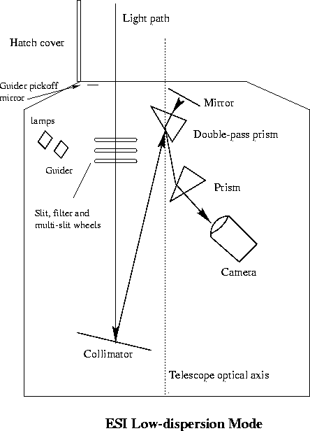


As can be seen in Figure 5, in low-D mode the full 2K x 4K of the CCD is not utilized. In principle a subwindow can be used, but this will not greatly decrease the readout time, hence the full CCD is generally read out in this mode. A standard setup (e.g. "LowD_1.0") can be used to select the low-D mode and a slit.
There is no need for order separation. Since the dispersion is done by prisms, there are no higher order spectra as there are with gratings or grisms.
Figure 5 is a schematic of the configuration for this mode.

Figure 5: Optical layout for the low-D configuration.
Figure 6 is a sample spectrum in raw CCD format and Figure 7 is an extracted spectrum of Wolf 1348 in the low-D mode. Both figures show spectra taken through the 6 arcsec-wide slit.

Figure 6: Low-D example spectrum [pixel (0,0) is at the upper left].

Figure 7: Wolf 1348 through the 6-arcsec slit.
Wavelength calibration in this mode uses the HgNe and Xe lamps. CuAr lamps will add more lines to the blue of the Xe lines, which is valuable for constraining the high-order fits required. Other Web pages provide plots of the different lamps and line lists. Rick White (STScI) has also kindly provided some IRAF output showing line identifications for the combined set of lamps.
Note that the wavelength calibration will vary with slit position. Mostly this will be a change in the wavelength zero-point, but there may be subtle effects in higher order terms as the distortions of the optical system become significant.
A polynomial fit of pixel to wavelength (or vice versa) will likely require terms as high as sixth order. Plotting (1/wavelength)^2 vs. pixel number is much more linear, but for an accurate fit still requires sixth order terms. Such high order polynomials require care when extrapolating the fits beyond the positions of wavelength calibration lines.


